Crossed Molecular Beams Method

Last updated
October 2023

CMB

The crossed molecular beam (CMB) technique is a well-established method for studying the dynamics of gas phase collisions and reactions. The basic methodology is to create two molecular beams containing the two colliders and direct these beams to intersect each other in a high vacuum chamber. By use of a detection method such as velocity map imaging (VMI) a great deal may be learnt about the resulting scattered molecules or reaction products, such as their kinetic energy and internal quantum state distributions, but the most important aspect of a CMB experiment is that it allows the determination of the dependence of these properties on the direction in which the molecules are scattered.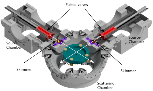

Schematic of CMB vacuum chambers — Fig. 1 - A slice through an engineering drawing of one of the CMB machines in the HWU lab. Molecular beams are formed in source chambers by expansion from pulsed valves. The source chambers are separated from the scattering chamber by bulkheads, with the only aperture at the tip of the skimmer. The resulting collimated molecular beams cross at right angles in the centre of the scattering chamber. In the CMB machines in the HWU lab, this crossing position is in the centre of the ion-optics of a VMI set-up, which extracts and velocity-maps ions produced by REMPI vertically, forming an image of the product scattered velocities.

This sensitivity to the spatial properties of a scattering process arises because the colliders are separately seeded in intersecting molecular beams, with narrow ranges of speeds and directions, so that the colliders approach one another along a well-defined direction in the laboratory with a well-defined centre of mass velocity, as illustrated in the diagram below. When considering a collision process it is useful to be able to view the system from the perspective of two frames of reference, the centre of mass frame, and the laboratory frame. The centre of mass frame is an axis system in velocity space having its origin at the centre of mass velocity of the collision system, while the origin of the laboratory frame is zero velocity with respect to the apparatus.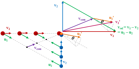

newton diagram — Fig. 2 - Two representations of a collision process. On the upper right hand side is a Newton diagram showing the key velocity vectors in a collision. v₁ and v₂ are the initial lab frame velocities of the two colliders. v_com and v_rel are the velocity of the centre of mass and the relative velocity respectively. u₁' and v₁' are, respectively, representative final centre-of-mass and laboratory frame velocities corresponding to a scattering angle θ. The lower left hand side shows snapshots of a collision process indicating the positions of the two colliders at different times, with the directions of the various lab and centre of mass frame velocities indicated. u₁ and u₂ are the initial and final relative velocities for the two colliders. The position of the centre of mass for each snapshot is indicated by a black dot. From the perspective of an observer at the centre of mass the colliders appear to approach one another from opposite directions and the collision occurs at this point.

Viewed from the centre-of-mass of the collision system, the molecules approach one another along the direction of their relative velocity vector v_rel and because of the azimuthal symmetry of the approach of colliders around this axis, the scattering is azimuthally symmetric around this axis. As a result of the collision, collider 1 has its velocity changed from u₁ to u₁' with a distribution of angles θ between these two vectors that is determined by the system’s reduced mass, relative speed distribution and the potential energy surface(s) describing the interactions between the two colliders. Since the relative velocity vector has a known, narrow distribution of magnitudes and directions in the laboratory frame this distribution may be inferred from the velocity distribution in the laboratory frame.

Examples of the distribution of final lab frame velocities for NO(A²Σ⁺; v = 0, N = 0) colliding with He measured using velocity map imaging are given below. These images are a two dimensional projection of the three dimensional velocity distribution arising from the scattering. Red indicates the greatest intensity, blue is lower intensity. The direction of the relative velocity vector is towards the lower left, with the scattering broadly symmetric around this axis. The animation shows a range of final rotational states, increasing in rotational energy in the NO product, from N' = 3 to N' = 10. Two things happen as N' increases, first the radius of the scattering ring decreases. This is a measurement of the speed of the scattered products: the total energy of the collision is fixed, and as additional energy is put into rotation of the NO, less is available for translation of the products, so they travel slower. The second observation is that the direction of the scattering changes, from the forward hemisphere, along the relative collision vector, to backwards (top right). This has a simple explanation in classical mechanics. Low-rotational states can be formed by collisions at a relatively long range, in 'glancing' impacts that result in only a small change in direction, and hence a small transfer of linear momentum into product rotational angular momentum. The faster product rotation implies a larger torque having been applied in the collision. A larger torque is applied by collisions along a line closer to the centre of mass of the NO, i.e. which have a smaller impact parameter. This more 'head on' collision generally results in more backscattering.